Deep Reinforcement Learning for Automated Stock Trading
Using reinforcement learning to trade multiple stocks through Python and OpenAI Gym | Presented at ICAIF 2020

This blog is based on our paper: Deep Reinforcement Learning for Automated Stock Trading: An Ensemble Strategy, presented at ICAIF 2020: ACM International Conference on AI in Finance.
Our codes are available on Github, and Our paper is available on SSRN.
If you want to cite our paper, the reference format is as follows:
Hongyang Yang, Xiao-Yang Liu, Shan Zhong, and Anwar Walid. 2020. Deep Reinforcement Learning for Automated Stock Trading: An Ensemble Strategy. In ICAIF ’20: ACM International Conference on AI in Finance, Oct. 15–16, 2020, Manhattan, NY. ACM, New York, NY, USA.
Overview
One can hardly overestimate the crucial role stock trading strategies play in investment.
Profitable automated stock trading strategy is vital to investment companies and hedge funds. It is applied to optimize capital allocation and maximize investment performance, such as expected return. Return maximization can be based on the estimates of potential return and risk. However, it is challenging to design a profitable strategy in a complex and dynamic stock market.
Every player wants a winning strategy. Needless to say, a profitable strategy in such a complex and dynamic stock market is not easy to design.
Yet, we are to reveal a deep reinforcement learning scheme that automatically learns a stock trading strategy by maximizing investment return.
Our Solution: Ensemble Deep Reinforcement Learning Trading Strategy
**This strategy includes three actor-critic based algorithms: Proximal Policy Optimization (PPO), Advantage Actor Critic (A2C), and Deep Deterministic Policy Gradient (DDPG).
It combines **the best features of the three algorithms, thereby robustly adjusting to different market conditions.
The performance of the trading agent with different reinforcement learning algorithms is evaluated using Sharpe ratio and compared with both the Dow Jones Industrial Average index and the traditional min-variance portfolio allocation strategy.
Part 1. Why do you want to use Deep Reinforcement Learning (DRL) for stock trading?
Existing works are not satisfactory. Deep Reinforcement Learning approach has many advantages.
1.1 DRL and Modern Portfolio Theory (MPT)
- MPT performs not so well in out-of-sample data.
- MPT is very sensitive to outliers.
- MPT is calculated only based on stock returns, if we want to take other relevant factors into account, for example some of the technical indicators like Moving Average Convergence Divergence (MACD), and Relative Strength Index (RSI), MPT may not be able to combine these information together well.
1.2 DRL and supervised machine learning prediction models
- DRL doesn’t need large labeled training datasets. This is a significant advantage since the amount of data grows exponentially today, it becomes very time-and-labor-consuming to label a large dataset.
- DRL uses a reward function to optimize future rewards, in contrast to an ML regression/classification model that predicts the probability of future outcomes.
1.3 The rationale of using DRL for stock trading
- The goal of stock trading is to maximize returns, while avoiding risks. DRL solves this optimization problem by maximizing the expected total reward from future actions over a time period.
- Stock trading is a continuous process of testing new ideas, getting feedback from the market, and trying to optimize the trading strategies over time. We can model stock trading process as Markov decision process which is the very foundation of Reinforcement Learning.
1.4 The advantages of deep reinforcement learning
- Deep reinforcement learning algorithms can outperform human players in many challenging games. For example, on March 2016, DeepMind’s AlphaGo program, a deep reinforcement learning algorithm, beat the world champion Lee Sedol at the game of Go.
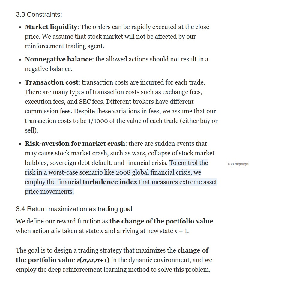
- **Return maximization **as trading goal: by defining the reward function as the change of the portfolio value, Deep Reinforcement Learning maximizes the portfolio value over time.
- The **stock market **provides sequential feedback. DRL can sequentially increase the model performance during the training process.
- The exploration-exploitation technique balances trying out different new things and taking advantage of what’s figured out. This is difference from other learning algorithms. Also, there is no requirement for a skilled human to provide training examples or labeled samples. Furthermore, during the exploration process, the agent is encouraged to explore the uncharted by human experts.
- Experience replay: is able to overcome the correlated samples issue, since learning from a batch of consecutive samples may experience high variances, hence is inefficient. Experience replay efficiently addresses this issue by randomly sampling mini-batches of transitions from a pre-saved replay memory.
- Multi-dimensional data: by using a continuous action space, DRL can handle large dimensional data.
- Computational power: Q-learning is a very important RL algorithm, however, it fails to handle large space. DRL, empowered by neural networks as efficient function approximator, is powerful to handle extremely large state space and action space.
Part 2: What is Reinforcement Learning? What is Deep Reinforcement Learning? What are some of the related works to use Reinforcement Learning for stock trading?
2.1 Concepts
Reinforcement Learning is one of three approaches of machine learning techniques, and it trains an agent to interact with the environment by sequentially receiving states and rewards from the environment and taking actions to reach better rewards.
Deep Reinforcement Learning approximates the Q value with a neural network. Using a neural network as a function approximator would allow reinforcement learning to be applied to large data.
Bellman Equation is the guiding principle to design reinforcement learning algorithms.
Markov Decision Process (MDP) is used to model the environment.
2.2 Related works
Recent applications of deep reinforcement learning in financial markets consider discrete or continuous state and action spaces, and employ one of these learning approaches: critic-only approach, actor-only approach, or and actor-critic approach.
Critic-only approach: the critic-only learning approach, which is the most common, solves a discrete action space problem using, for example, Q-learning, Deep Q-learning (DQN) and its improvements, and trains an agent on a single stock or asset. The idea of the critic-only approach is to use a Q-value function to learn the optimal action-selection policy that maximizes the expected future reward given the current state. Instead of calculating a state-action value table, DQN minimizes the mean squared error between the target Q-values, and uses a neural network to perform function approximation. The major limitation of the critic-only approach is that it only works with discrete and finite state and action spaces, which is not practical for a large portfolio of stocks, since the prices are of course continuous.
Q-learning: is a value-based Reinforcement Learning algorithm that is used to find the optimal action-selection policy using a Q function.
DQN: In deep Q-learning, we use a neural network to approximate the Q-value function. The state is given as the input and the Q-value of allowed actions is the predicted output.
Actor-only approach: The idea here is that the agent directly learns the optimal policy itself. Instead of having a neural network to learn the Q-value, the neural network learns the policy. The policy is a probability distribution that is essentially a strategy for a given state, namely the likelihood to take an allowed action. The actor-only approach can handle the continuous action space environments.
Policy Gradient: aims to maximize the expected total rewards by directly learns the optimal policy itself.
Actor-Critic approach: The actor-critic approach has been recently applied in finance. The idea is to simultaneously update the actor network that represents the policy, and the critic network that represents the value function. The critic estimates the value function, while the actor updates the policy probability distribution guided by the critic with policy gradients. Over time, the actor learns to take better actions and the critic gets better at evaluating those actions. The actor-critic approach has proven to be able to learn and adapt to large and complex environments, and has been used to play popular video games, such as Doom. Thus, the actor-critic approach fits well in trading with a large stock portfolio.
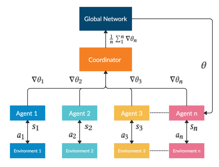
A2C: A2C is a typical actor-critic algorithm. A2C uses copies of the same agent working in parallel to update gradients with different data samples. Each agent works independently to interact with the same environment.
PPO: PPO is introduced to control the policy gradient update and ensure that the new policy will not be too different from the previous one.
DDPG: DDPG combines the frameworks of both Q-learning and policy gradient, and uses neural networks as function approximators.
Part 3: How to use DRL to trade stocks?
3.1 Data
We track and select the Dow Jones 30 stocks (at 2016/01/01) and use historical daily data from 01/01/2009 to 05/08/2020 to train the agent and test the performance. The dataset is downloaded from Compustat database accessed through Wharton Research Data Services (WRDS).
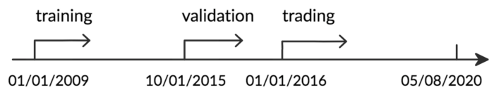
The whole dataset is split in the following figure. Data from 01/01/2009 to 12/31/2014 is used for training, and the data from 10/01/2015 to 12/31/2015 is used for validation and tuning of parameters. Finally, we test our agent’s performance on trading data, which is the unseen out-of-sample data from 01/01/2016 to 05/08/2020. To better exploit the trading data, we continue training our agent while in the trading stage, since this will help the agent to better adapt to the market dynamics.
class StockEnvTrain(gym.Env):
“””A stock trading environment for OpenAI gym”””
metadata = {‘render.modes’: [‘human’]}
def __init__(self, df, day = 0):
self.day = day
self.df = df
# Action Space
# action_space normalization and shape is STOCK_DIM
self.action_space = spaces.Box(low = -1, high = 1,shape = (STOCK_DIM,))
# State Space
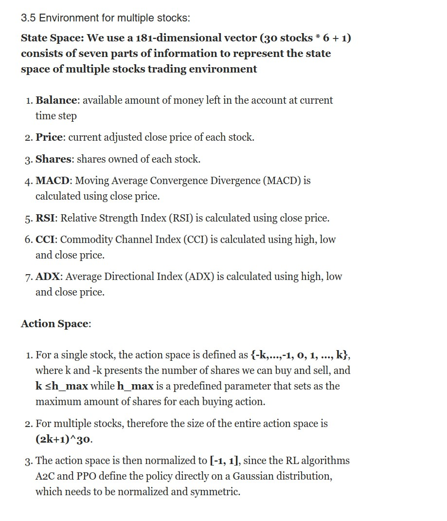
# Shape = 181: [Current Balance]+[prices 1–30]+[owned shares 1–30]
# +[macd 1–30]+ [rsi 1–30] + [cci 1–30] + [adx 1–30]
self.observation_space = spaces.Box(low=0, high=np.inf, shape = (181,))
# load data from a pandas dataframe
self.data = self.df.loc[self.day,:]
self.terminal = False
# initalize state
self.state = [INITIAL_ACCOUNT_BALANCE] + \
self.data.adjcp.values.tolist() + \
[0]*STOCK_DIM + \
self.data.macd.values.tolist() + \
self.data.rsi.values.tolist() + \
self.data.cci.values.tolist() + \
self.data.adx.values.tolist()
# initialize reward
self.reward = 0
self.cost = 0
# memorize all the total balance change
self.asset_memory = [INITIAL_ACCOUNT_BALANCE]
self.rewards_memory = []
self.trades = 0
#self.reset()
self._seed()
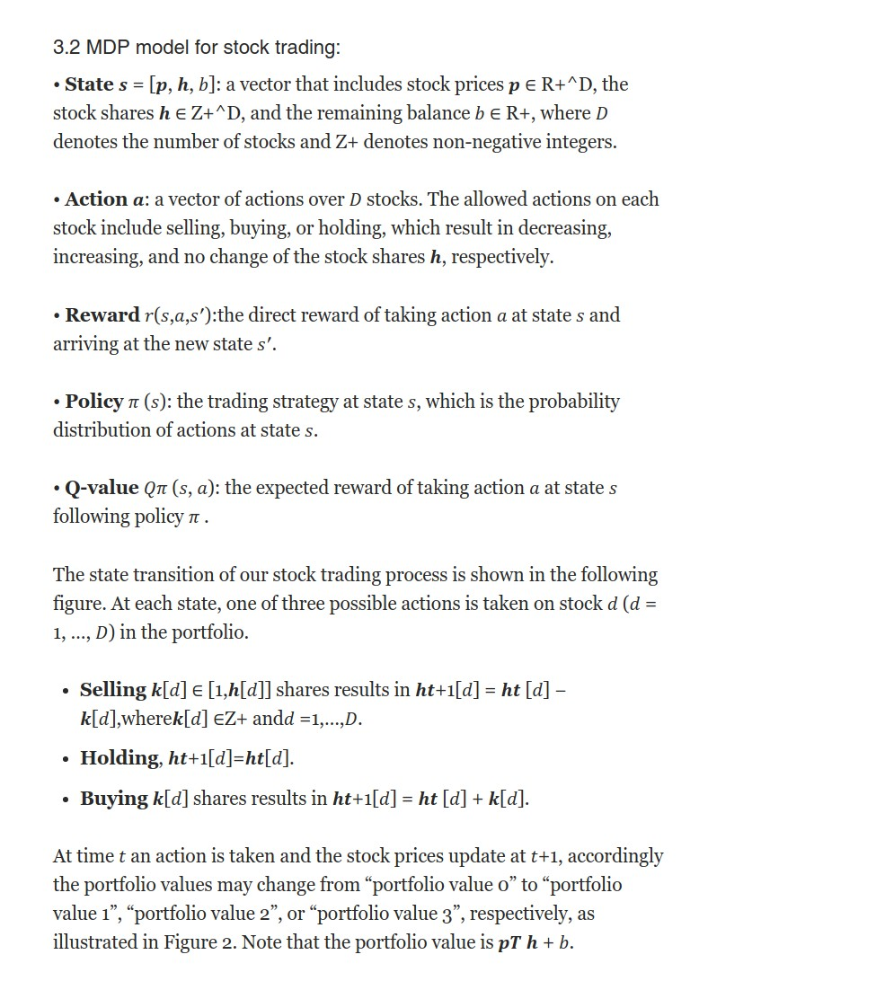
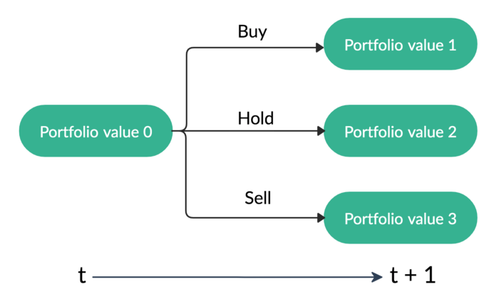
3.6 Trading agent based on deep reinforcement learning
A2C
A2C is a typical actor-critic algorithm which we use as a component in the ensemble method. A2C is introduced to improve the policy gradient updates. A2C utilizes an advantage function to reduce the variance of the policy gradient. Instead of only estimates the value function, the critic network estimates the advantage function. Thus, the evaluation of an action not only depends on how good the action is, but also considers how much better it can be. So that it reduces the high variance of the policy networks and makes the model more robust.
A2C uses copies of the same agent working in parallel to update gradients with different data samples. Each agent works independently to interact with the same environment. After all of the parallel agents finish calculating their gradients, A2C uses a coordinator to pass the average gradients over all the agents to a global network. So that the global network can update the actor and the critic network. The presence of a global network increases the diversity of training data. The synchronized gradient update is more cost-effective, faster and works better with large batch sizes. A2C is a great model for stock trading because of its stability.
DDPG

DDPG is an actor-critic based algorithm which we use as a component in the ensemble strategy to maximize the investment return. DDPG combines the frameworks of both Q-learning and policy gradient, and uses neural networks as function approximators. In contrast with DQN that learns indirectly through Q-values tables and suffers the curse of dimensionality problem, DDPG learns directly from the observations through policy gradient. It is proposed to deterministically map states to actions to better fit the continuous action space environment.
PPO
We explore and use PPO as a component in the ensemble method. PPO is introduced to control the policy gradient update and ensure that the new policy will not be too different from the older one. PPO tries to simplify the objective of Trust Region Policy Optimization (TRPO) by introducing a clipping term to the objective function.
The objective function of PPO takes the minimum of the clipped and normal objective. PPO discourages large policy change move outside of the clipped interval. Therefore, PPO improves the stability of the policy networks training by restricting the policy update at each training step. We select PPO for stock trading because it is stable, fast, and simpler to implement and tune.
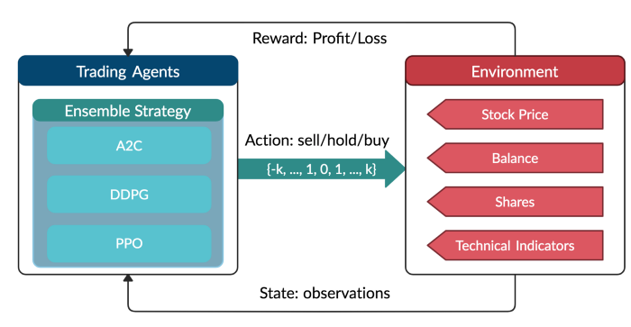
Ensemble strategy
Our purpose is to create a highly robust trading strategy. So we use an ensemble method to automatically select the best performing agent among PPO, A2C, and DDPG to trade based on the Sharpe ratio. The ensemble process is described as follows:
Step 1. We use a growing window of 𝑛 months to retrain our three agents concurrently. In this paper, we retrain our three agents at every three months.
Step 2. We validate all three agents by using a 3-month validation rolling window followed by training to pick the best performing agent which has the highest Sharpe ratio. We also adjust risk-aversion by using turbulence index in our validation stage.
Step 3. After validation, we only use the best model with the highest Sharpe ratio to predict and trade for the next quarter.
from stable_baselines import SAC
from stable_baselines import PPO2
from stable_baselines import A2C
from stable_baselines import DDPG
from stable_baselines import TD3
from stable_baselines.ddpg.policies import DDPGPolicy
from stable_baselines.common.policies import MlpPolicy
from stable_baselines.common.vec_env import DummyVecEnv
def train_A2C(env_train, model_name, timesteps=10000):
 “””A2C model”””
 start = time.time()
 model = A2C(‘MlpPolicy’, env_train, verbose=0)
 model.learn(total_timesteps=timesteps)
 end = time.time()
 model.save(f”{config.TRAINED_MODEL_DIR}/{model_name}”)
 print(‘Training time (A2C): ‘, (end-start)/60,’ minutes’)
 return model
def train_DDPG(env_train, model_name, timesteps=10000):
 “””DDPG model”””
 start = time.time()
 model = DDPG(‘MlpPolicy’, env_train)
 model.learn(total_timesteps=timesteps)
 end = time.time()
 model.save(f”{config.TRAINED_MODEL_DIR}/{model_name}”)
 print(‘Training time (DDPG): ‘, (end-start)/60,’ minutes’)
 return model
def train_PPO(env_train, model_name, timesteps=50000):
 “””PPO model”””
 start = time.time()
 model = PPO2(‘MlpPolicy’, env_train)
 model.learn(total_timesteps=timesteps)
 end = time.time()
 model.save(f”{config.TRAINED_MODEL_DIR}/{model_name}”)
 print(‘Training time (PPO): ‘, (end-start)/60,’ minutes’)
 return model
def DRL_prediction(model, test_data, test_env, test_obs):
 “””make a prediction”””
 start = time.time()
 for i in range(len(test_data.index.unique())):
   action, _states = model.predict(test_obs)
   test_obs, rewards, dones, info = test_env.step(action)
   # env_test.render()
 end = time.time()
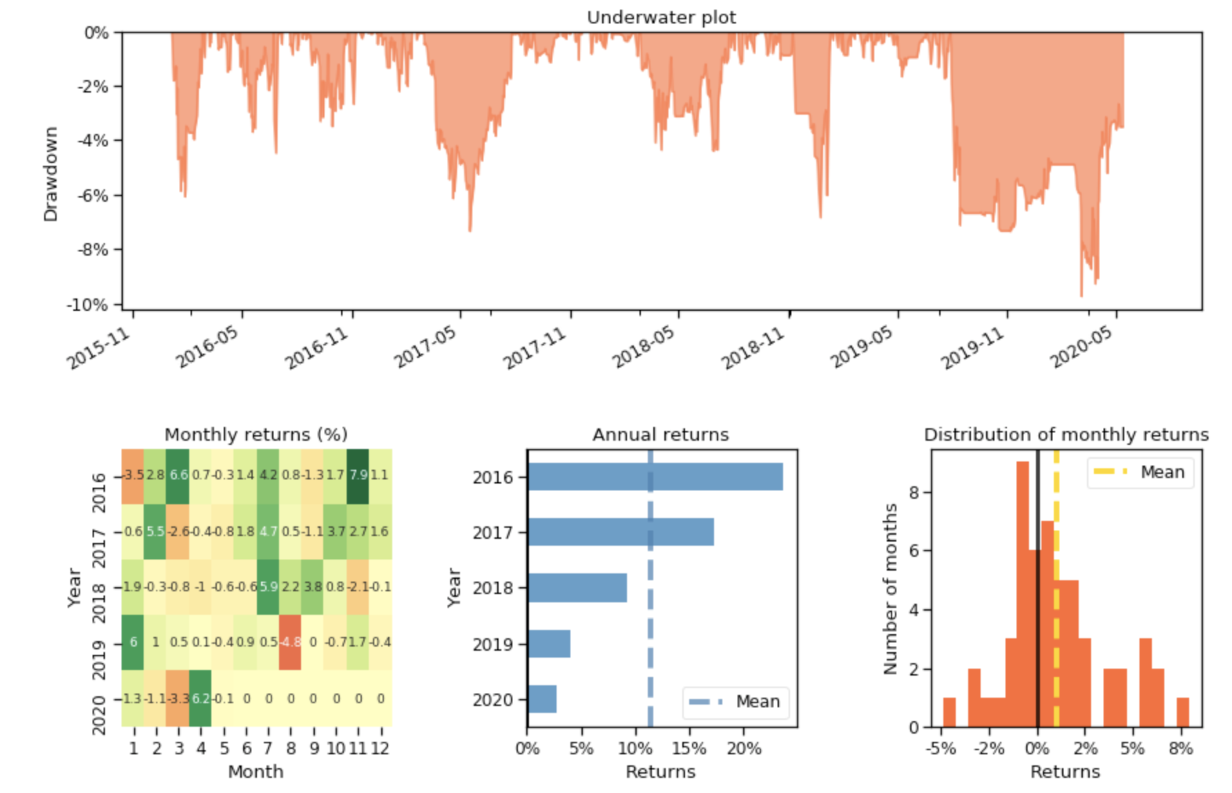
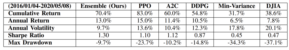
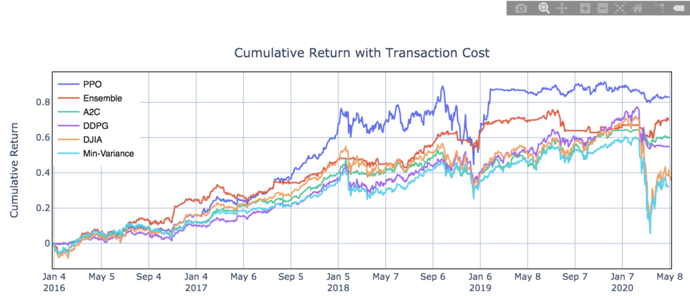
3.7 Performance evaluations